Contents
Goal
In this example, we’ll pretend we are investigating the effects of seed density on a run. We will add (concentrated) media in order to control osmo at a fixed point, and do the same with glucose. This is also the first time we’ve run this cell line – so we don’t know optimal conditions or how well they’ll grow.
Setup
The most important part of simulating a run is the setup; I’m going to walk through each part of the setup here and explain how it works. We use create_config in main.py for ease of use.
def create_config(num_experiments,
                  cell_line = None,
                  glucose_sp = Q(1.5, 'g/L'),
                  seed_density = Q(10, 'e5c/ml'),
                  equipment_instances = None):
  start_time = np.datetime64('2020-01-01')
  initial_volume = Q(0.5, 'L')
  seed_density = seed_density
  starting_cells = initial_volume*seed_density
We start by adding seed_density as an input and defining a few quantities that we will use throughout the configuration; the initial volume and seed density will need to be passed to multiple things like bioreactor setup or control strategies (they use these numbers in their calculations for predicted VCD and consumption). ‘Q’ creates a quantity; Q(0.5, 'L') means 0.5 litres.
From here, we will be passing arguments to each of the wrappers for assays, controls, environment, and cells. The default values in CC-Sim are for a 2L bioreactor, and we only need to pass arguments that are required or that we want to change from the default. As an example, here are the default values for the bioreactor setup (bioreactor.py):
                 start_time,
                 initial_components,
                 seed_volume,
                 initial_temperature,
                 volume = Q(3, 'L'),
                 agitator = agitator(),
                 diameter = Q(13, 'cm'),
                 sparger_height = Q(2, 'cm'), # Height from bottom of vessel
                 sparger_pore_size = Q(20, 'um'),
                 cell_separation_device = None,     # Perfusion only
                 head_pressure = Q(760, 'mmHg'),
                 heat_transfer_coeff = Q(50, 'W/m**2'), #per degree (not supported)
Since we are fine with the default values, we only have to specify the first 4 arguments:
  media = helper_functions.create_media_as_mole(example_media, initial_volume)
  br_setup = {'start_time':start_time,
              'initial_components':media,
              'seed_volume':initial_volume,
              'initial_temperature':36,
              }
We pass the start time (as numpy.datetime64), along with the moles of each component in the bioreactor – which we create from a function that takes the media definition and the volume.
  assay_setup = {**equipment_instances,
                 'start_time':start_time,
                 'bioHT_list':['glucose', 'IGG'],
                 }
The assays wrapper takes the same start time along with instances of a shared equipment like osmo machine, BGA, cell counter, and bioHT. We must pass instances of shared equipment so that all experiments share the same systematic bias. For the programmers, we passed the instantiated object itself rather than a class. We also pass ['glucose', 'IGG'], which are the assays that we want the bioHT to run every offline sample. The input arguments can be looked up under wrapper of assays.py.
  glucose_feed = (controls.basic_fed_batch_feed,[],
                    {'feed_mixture':{'glucose': Q(500, 'g/L')},
                    'initial_volume':initial_volume,
                    'sample_interval':Q(24, 'h'),
                    'cpp':'glucose',
                    'set_point':glucose_sp,
                    'initial_time': start_time,
                    'target_seeding_density':seed_density}
                  )
Here begins the controls configuration, starting with glucose. The controls wrapper takes a list of tuples in form (control strategy, *args, **kwargs). The type of control strategy employed here is controls.basic_fed_batch_feed, which attempts to predict consumption of the given critical process parameter based on how VCD is trending. It attempts to move concentration to the setpoint at the end of sample interval.
It is called “basic” because it isn’t very smart about predictions: it basically just extrapolates from what happened the previous day.
This configuration supplies the simulation with everything it needs to know in order to create the control, including what media to make, what actuation device to use, and how it is predicting the necessary flowrate. Premade control strategies and their input arguments can be looked up in controls.py.
  concentrated_feed = (controls.basic_fed_batch_feed, [],
                        {'feed_mixture':example_concentrated_media,
                        'initial_volume':initial_volume,
                        'sample_interval':Q(24, 'h'),
                        'cpp':'mOsm',
                        'set_point':Q(330, 'mM'),
                        'initial_time': start_time,
                        'target_seeding_density':seed_density,
                        'max_added':Q(1., 'L'),}
                      )
This configuration is just like glucose feed, except that we are controlling based off of osmo and have a concentrated media that we are adding.
   aeration_setup = (controls.aeration,[],
                    {'setpoint':60, 'max_air':Q(0.2, 'L/min'),
                    'max_O2':Q(0.1, 'L/min'),}
                    )
Aeration, pH, and temperature also have their own controls. We define aeration separately simply because the kwargs we are passing are verbose.
  control_setup = [glucose_feed,
                   aeration_setup,
                   (controls.temperature, [36], {}),
                   (controls.pH, [7.15], {}),
                   concentrated_feed,
                   ]
  cell_setup = {'cell_line':cell_line,
                'seed_cells':starting_cells}
We take all of the controls (along with the tmperature and pH we defined inline) and make a list to be passed to the simulation.
config = (assay_setup, control_setup, br_setup, cell_setup)
return [config]*num_experiments
Lastly, we package the entire configuration into a tuple, and make a list of the same entry for each experiment we wanted to run. If we wanted to configure the experiments differently, we could create separate configurations and make a list of the configurations (e.g. [config1, config2, etc...]. I prefer to just make and run a separate configuration file for each because it is easier to keep the metrics I want to plot later separate that way.
  shared_equipment = {'osmo':assays.osmo(),
                      'BGA_instance':assays.BGA(),
                      'cell_counter':assays.cell_counter(),
                      'bioHT':assays.bioHT(),}

  cell_line = cell_sim.gen_cell_line()
  low_config = create_config(2,
                             cell_line = cell_line,
                             equipment_instances = shared_equipment,
                             seed_density = Q(2, 'e5c/ml'),
                             )
  medium_config = create_config(2,
                             cell_line = cell_line,
                             equipment_instances = shared_equipment,
                             seed_density = Q(5, 'e5c/ml'),
                             )
  high_config = create_config(2,
                             cell_line = cell_line,
                             equipment_instances = shared_equipment,
                             seed_density = Q(10, 'e5c/ml'),
                             )
Finally, we create three separate configurations (each in duplicate) for the seeding densities we are interested in.
Running the Simulation
Once we have are experimental configuration defined, we pass this to the simulation and let it run. We call run_experiments on the list of configurations we just created. The simulation will return metrics.
  low_metrics = run_experiments(low_config)
  medium_metrics = run_experiments(medium_config)
  high_metrics = run_experiments(high_config)
Visualizing our Results
CC-Sim includes a couple of functions to make it easy to look at the metrics of interest and plot them. The simplest is dual_plot, which takes two variables we would like to plot along with the metrics and plots it for us. We can figure out what variables are available for plotting by calling low_metrics[0][0].keys(), which takes the first experiment (specified by the first [0]), then the first datapoint (the second [0]), and prints all of the keys in it. The first datapoint also contains all offline assays. It returned:
dict_keys(['glucose feed rate', 'glucose addition rate', 'aeration_PID', 'heating_PID', 'pH_PID', 'mOsm feed rate', 'mOsm addition rate', 'time', 'pH', 'dO2', 'temperature', 'mass', 'BGA_dO2', 'BGA_pH', 'BGA_dCO2', 'glucose', 'IGG', 'VCD', 'cell_diameter', 'viability', 'mOsm', 'limiting_rate', 'target_diameter', 'growth_inhibition', 'extinction_rate', 'amino_acids', 'dCO2', 'rVCD', 'rglucose', 'compA', 'total_cell_volume', 'total_living_cells'])
Since realistic_mode is turned off in the global simulation settings, we are getting metrics that we would get in real life (‘glucose’) as well as “cheater metrics” like ‘rglucose’ that the simulation is returning that allow us to cheat and access the underlying numbers from the simulation. Cheater metrics are both 100% accurate (no assay error) and not limited to offline assays.
When comparing multiple runs with different conditions, I prefer to make two plots, each containing two variables, so that I can easily look at how 4 variables progressed for a condition and keep them together. dual_subplot is called and passed the four variables I am interested in plotting, along with titles to make clear what we’re looking at:
dual_subplot('viability', 'VCD', 'mOsm', 'IGG', metrics = low_metrics,
             big_title = r'Seed Density: 2 e5c/ml', left_title = 'Viability vs VCD',
             right_title = 'Osmo vs IGG')
When looking at these, I notice a few trends:
- The higher the seed density, the earlier the VCD peak
- The higher the seed density, the deeper the crash in death phase
- The lowest seed density starts producing IGG later and doesn’t get to the same level before being harvested
- The feed strategy tends to alternate between over-and-undershooting
The first three are somewhat to be expected, and the last could warrant further investigation (although it’s probably because we used basic_fed_batch_feed as the strategy, and had no historical data to feed by).
One thing we didn’t look at is what our final volume was, which we should probably do.
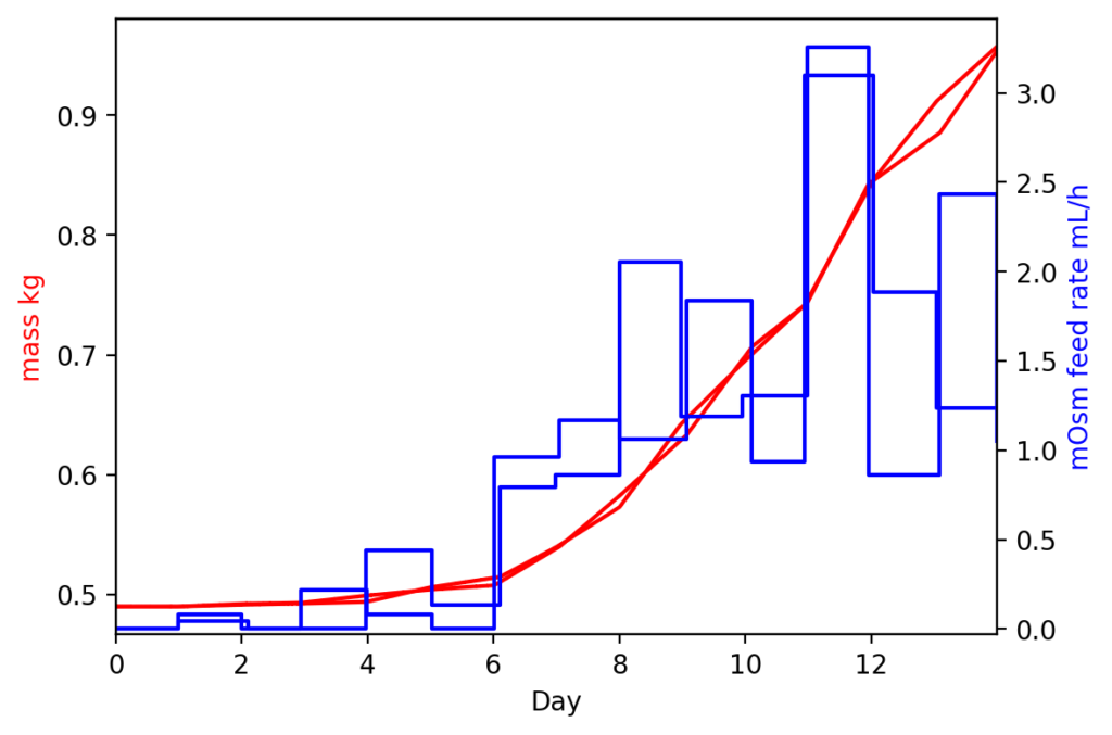
  dual_plot('mass', 'mOsm feed rate', metrics = low_metrics)
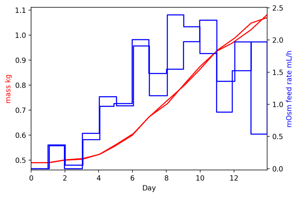
  dual_plot('mass', 'mOsm feed rate', metrics = high_metrics)

As we might expect, the lower seed density both took longer to start adding media and had less total added at harvest time (note that mass is the left axis).
It would be similarly trivial to graph glucose levels, oxygen levels, pH, and other metrics in the same manner.


